McDANIEL (KP Engineering, LP)  

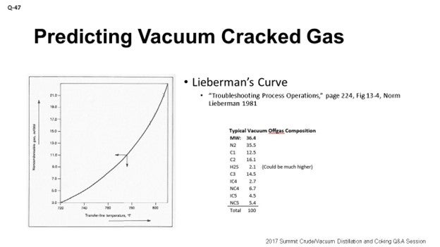
My direct response is that one of the tools I utilize when I am looking at either modeling an existing unit or a new design is Lieberman’s Curve. It is readily available in Norman Lieberman’s book, Troubleshooting Process Operations, as well as several other books. Most everyone here is probably familiar with the curve. It is a representation of the number of scuffs of off gas per feed to the vacuum unit. Mind you, this is total off-gas of non-condensable off the hot well. It is a general curve that works well when trying to determine how much off-gas you will have, and it fits well to a 13 API typical vacuum charge. 

If you are running a light sweet crude, then, yes, you tend to trend below the line. If you are running a heavy sour crude, you tend to trend above the curve. One of the solutions I suggest is one that I have seen some folks do and which is what I heard from the Operations folks to whom I spoke when I was researching my response. This solution is actually to take some of the empirical data from your plant, get your off-gas compositions and off-gas rates, and then chart them on the same curve. Be sure that you are doing it for applicable similar crude slates. If you do use comparable data, then you will be able to create a similar set of curves – on this same Lieberman’s Curve – that address different crude slates and API vacuum charge rates. When I have used this curve, my results tend to go along well with the refineries with which I am working, regarding what I am modeling versus what I am actually seeing in the base case data. 

 

 

 

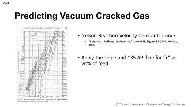
Another option that you can consider, as did one of my co-workers, is actually to look at the Nelson’s Reaction Velocity Constant Curve which deals more with direct cracking for specific products. My co-worker was trying to find a way to apply something that Lieberman’s Curve does not address – that is, time. Because what are the two key parameters of cracking? Time and temperature. This Nelson Reaction Velocity Constants curve takes into account both time and temperature. Through trial and error, my co-worker found that when using the slope of the curve, most of these products (lines) were very similar, with all of them going along about the 35 API line, as shown on the slide. It the line second to the left. Doug could follow along in line with a typical vacuum unit charge, which allowed him to then back-calculate the equation shown on the Nelson Reaction Velocity Constants curves for the case of T and actually solve for X as a weight percent of vacuum charge. That calculation actually allowed us to break up the transfer line into segments, so we could see how much cracking was happening as we were progressing and feeding into the vacuum column. It is a unique application which is a little out of the box, but it has worked well and is just another option. I know there are lots of correlations or options of which you guys may be aware as well, and I would love to hear about them. 

 

 

 

SOLOMON (Athlon Solutions)  

Ross gave a very complete answer. In the essence of time here, since we are getting close to 11:30 already, let’s just leave it there. 

  

GRANT NICCUM (Process Consulting Services Inc.) 

I just want to point out that the risk associated with underestimating the cracked gas rate is much higher than the risk when overestimating it. If you have some extra capacity in your vacuum system, then utilities consumption cooling water and steam will be a bit higher than optimum. However, the system should still work well. If you underestimate the cracked gas rate in your vacuum system design, you will run with broken ejectors, have high tower operating pressure, and miss your vacuum resid cutpoint. Therefore, underestimating the cracked gas rate has a large downside. 

In a modern wet vacuum system, the first-stage ejector and first stage intercondenser are responsible for the majority of the total system cost. The majority of the load to the first-stage ejector and intercondenser is made up of stripping steam, heater velocity steam, and condensable hydrocarbons. Cracked gas comprises a small percentage – maybe 10% – of the first-stage load and therefore has a small impact on total system cost. The cracked gas rate becomes significant in the downstream second- and third-stage ejectors and condensers where higher-than-design cracked gas rates can cause instabilities that ultimately affect the first-stage ejectors and the tower pressure. The second- and third-stage ejectors and condensers are small compared to the first-stage equipment, so the extra capacity that results from moderately overestimating the cracked gas rate does not cost a lot but does contribute significantly to overall system stability.  

 

McDANIEL (KP Engineering, LP) 

Grant made a good point. Operators have to understand that if you are using these curves to get the overall off gas. Then, if you are trying to determine what your loads are to your jets, you will have to take into account the rest of the vacuum system. If the vacuum column has significant gas production, stripping steam, or velocity steam in the heater, it will increase the jet sizing. 

 

KEVIN SOLOMON (Athlon Solutions) 

In the past, vacuum towers’ flash zones have operating at or below atmospheric tower flash zone temperatures. These units relied on the vacuum to increase heavy gasoil yields from the atmospheric resid without running the risk of thermal cracking associated with higher temperatures. The new design “deep cut” vacuum units have reduced the potential for coking in the furnace and tower bottoms; and now, flash zone temperatures are in the range of thermal cracking. Some units see vacuum unit flash temperatures 100 to 150°F higher than the atmospheric tower. This elevated temperature creates unique problems in the overhead water. You can see increased levels of chlorides in the vacuum overhead water since the increased temperature allows for increased chloride hydrolysis. We also see higher levels of ammonia be produced in-situ from nitrogen compounds in the reduced crude. 

  

W. ROSS McDANIEL (KP Engineering) 

A well-known and widely available correlation is Norman Lieberman’s curve, which is shown here presented in Troubleshooting Process Operations as Figure 13-4. Norm gives a relationship of the amount of full-range vacuum off-gas [in scf/bbl (standard cubic foot per barrel) of vacuum charge] to heater outlet transfer line temperature [in degrees Fahrenheit]. 

 

Lieberman’s Curve2

The curve represents empirical data from multiple units with common crude slate feeds. This scf/bbl value of non-condensables represents the full range of vacuum off-gas. It can be converted to a total wt% of vacuum charge and then a typical off-gas component breakdown, or the breakdown supplied by the specific refinery sample can be applied to the total off-gas. This is how I typically do vacuum simulations. Below is a typical component breakdown for an off gas with a 36.4 MW. 

TYPICAL VACUUM OFF-GAS COMPOSITION
	MW:	36.4
	N2	35.5
	C1	12.5
	C2	16.1
	H2S	2.1	(Could be much higher)
	C3	14.5
	IC4	2.7
	NC4	6.7
	IC5	4.5
	NC5	5.4
	Total	100

 

It has been shown that this curve fits well to a typical API 13 vacuum tower charge, but opportunity light sweet crudes fall below the curve and more heavy sour crudes trend above the Lieberman’s Curve. One way to improve this curve for your facility is to take the curve and apply your facility’s own historical data on the curve for a similar crude diet. Another reference for cracking is “Nelson’s Reaction Velocity Constants Curve”3.  

 

The Nelson curve is applied more to cracking for specific products, but it does consider the relationship not addressed in Lieberman’s curve, which is time. The two key parameters to cracking are both the temperature and time that are applied to the feedstock. My coworker, Doug McDaniel, used the approximate slope of these curves to develop an applicable curve for typical vacuum feed, which happens to fall at around 35 API product gravity on this graph. Rearrange the y-axis formula to solve for x, in terms of wt%. The equation can could then be applied to vacuum heater and transfer line segments to determine a total cumulative wt% cracked of the original vacuum feed. 

I am sure others can point you to different correlations, but the key is to make sure you are considering your desired feedstock and other conditions on your vacuum column – such as whether the column is dry or wet – when using your results to size or rate your overhead vacuum system.